Evaluating Solutions

To evaluate solutions for self-adaptation, we consider the achieved utility for the adaptable software and the execution time of the solution to perform self-adaptation resolving the issues injected into the CompArch model. Thus, developers can evaluate the effectiveness (in terms of the achieved utility for the adaptable software) and efficiency (in terms of execution time) of their self-adaptation solutions.

Moreover, by increasing the size of the architecture (and thus, the size of the CompArch model) and the number of issues injected per simulation round, the scalability of adaptation engines can be evaluated with respect to effectiveness and efficiency. For this purpose, we provide a generator for mRUBiS architectures with user-defined numbers of shops/tenants to obtain various sizes of the CompArch model.

After a simulation has finished, simulator.showResults(); can be invoked so that the simulator stores the simulation results into the folder results of the Eclipse project (refresh the folder in Eclipse after the simulation to see the created files containing the results). The results comprise the utility of the adaptable software and the execution time of the feedback loop.

Utility of the Aadaptable Software

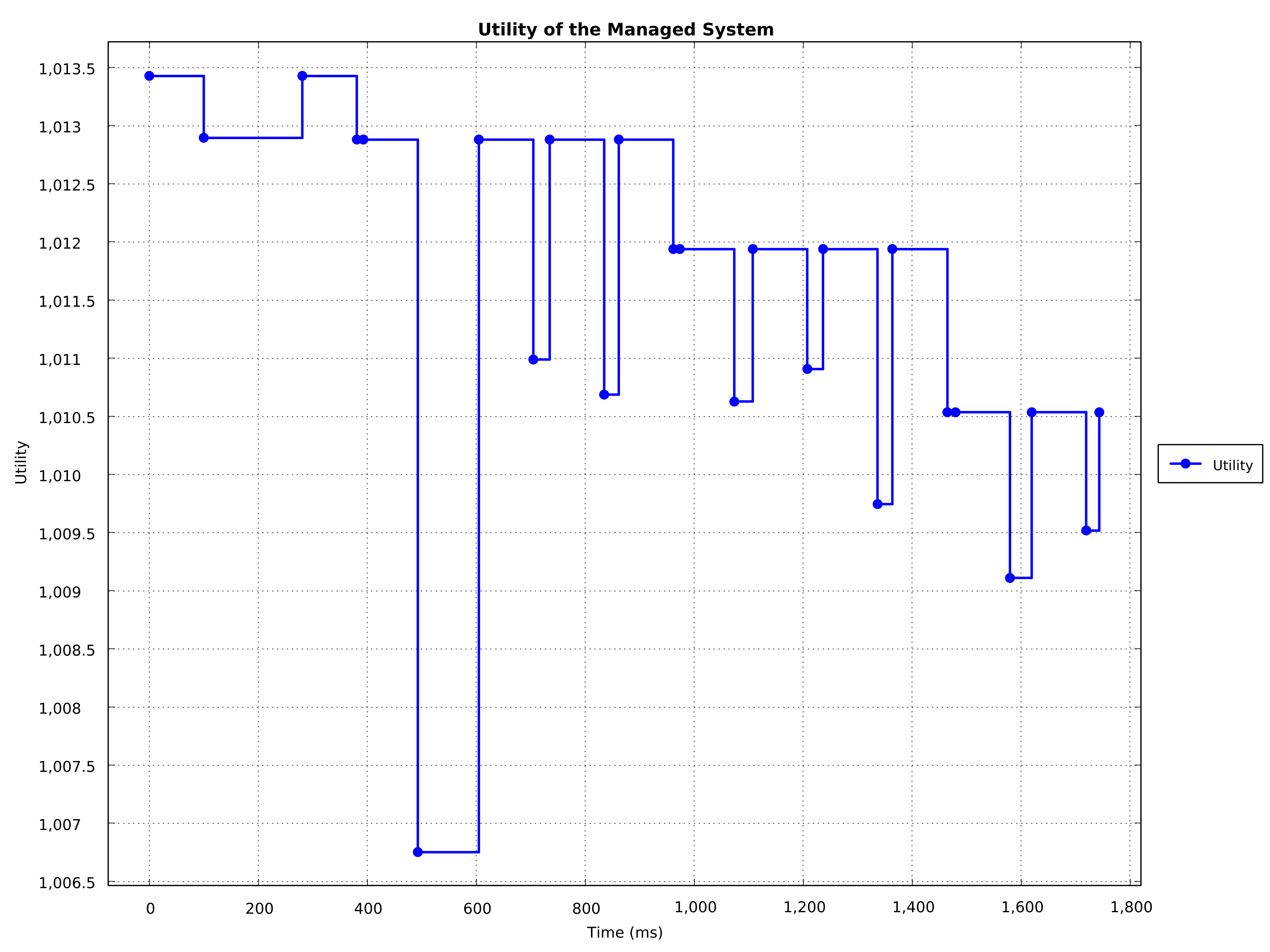
The utility of the adaptable software is computed and measured over the time of the simulation using the given utility function and presented by a step chart. The raw data is also provided in a csv file.

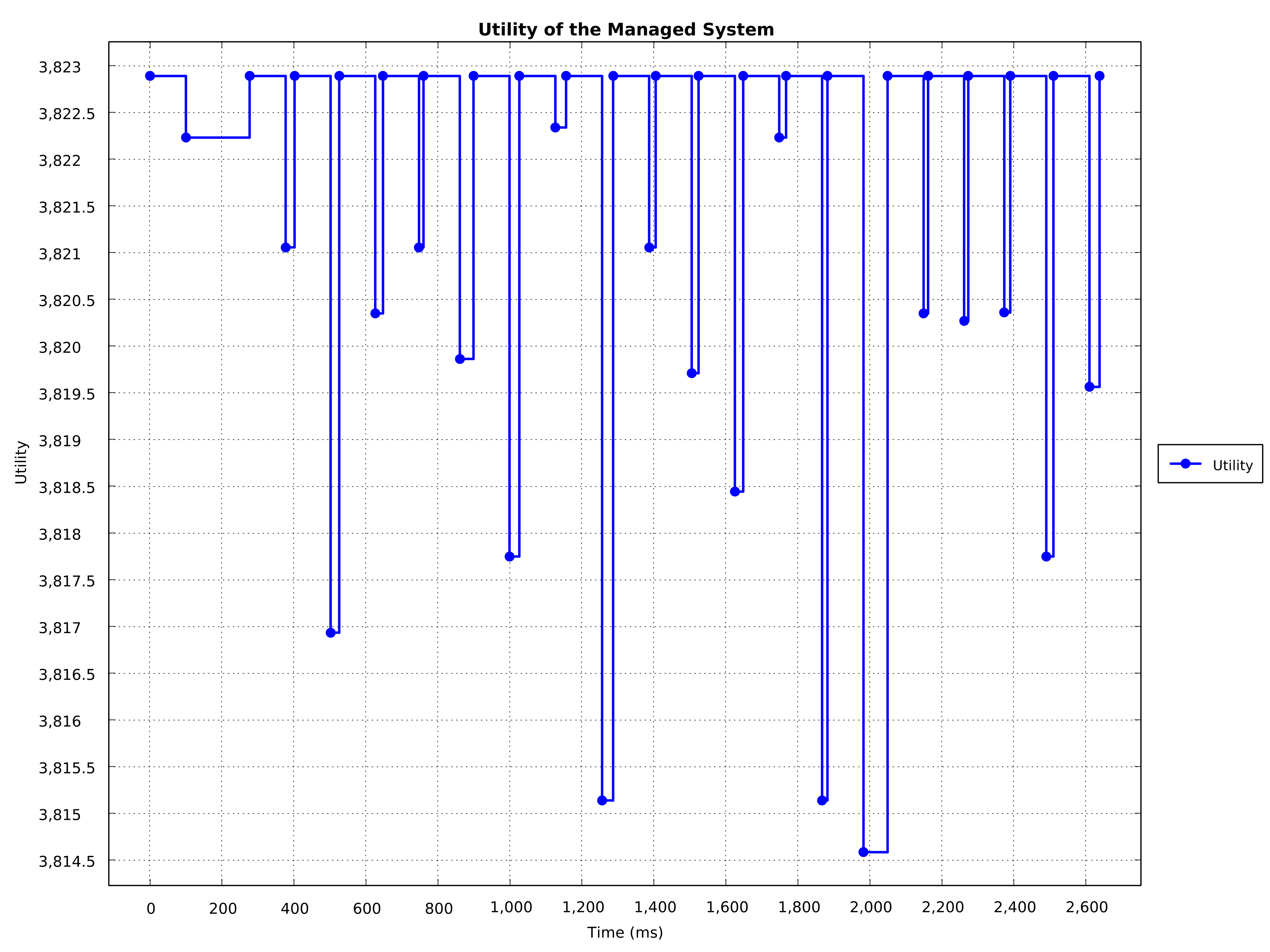
Each drop in the utility is caused by issues that are injected by the simulator into the CompArch model. Each increase of the utility is achieved by self-adaptation that successfully resolves the issues. In this case, the self-adaptation was able to address all injected issues.

In contrast the following chart shows a case in which the self-adaptation was not able to address all injected issues. Consequently, the utility is decreasing in various steps, in this specific case three steps since three issues could not be resolved.

Differences between self-adaptation solutions are that some solutions...

• might not be able to address all issues. In this case, the drop of the utility caused by the issue cannot be compensated by a self-adaptation.
• might perform a self-adaptation faster than another solution. In this case, the increase of the utility is achieved earlier.
• might perform a "better" self-adaptation than another solution. For instance, when replacing a faulty component (i.e., one that is affected by an issue) of type A with a component of type B that is more reliable than A, instead of replacing it with a new instance of A, then the increase of the utility achieved by self-adaptation can be larger due to the better reliability of the replacing component. In this case, the increase of the utility can be larger for one self-adaptation option than for another option.

Therefore, the reward as the utility over time should be considered as well when evaluating different self-adaptation solutions.

Execution Time of the Self-Adaptation

The execution time of the self-adaptation is monitored for each simulation round, thus for each run of the adaptation engine's feedback loop, and presented as a chart. The raw data is also provided in a csv file.

The first run of the feedback loop typically takes more time than the other runs due to (Java) initialization costs.

Logging Report

Finally, the simulator logs information to a file (see Simulator.log in the results folder) and optionally to the console. After each simulation round, a report is logged. An example is shown below.

=============================================================================
Round: 20
Identified issues: 0
Current utility: 3822.8942 (+3.3269)
Execution time of the last feedback loop run in ms: 28
Total feedback loop execution time in ms: 628
Average feedback loop execution time per round in ms: 31
Standard deviation of the feedback loop execution time per round in ms: 36.7839
Total delay time in ms: 2002
=============================================================================

• Round refers to the current simulation round.
• Identified issues refers to the number of issues identified by the validators when validating the self-adaptation and the CompArch model.
• Current utility refers to the current utility of the managed system (see fist section of this page) and the difference to the previous computation of the utility after issues have been injected. In this case, the self-adaptation addresses some or all of the injected issues so that the utility increased by 3.3269.
• The next two lines refer to the execution time of the feedback loop for the very last run of the feedback loop and to the sum of the execution times of the feedback loop over all runs so far (in this case, the sum over the 20 runs of the feedback loop = 20 simulation rounds).
• The next line shows the standard deviation for the execution time of the feedback loop for each run.
• The last line refers to the sum of the delays that are performed by the simulator each time after a feedback loop has finished execution and before new issues are injected into the CompArch model. This delay can be configured when instantiating the simulator (see Using the Simulator).