Last updated Summer 2024 for Gephi version 0.10.1
This tutorial provides an introduction to Gephi, an open source tool for visualizing graphs / networks. It is commonly used for data analysis and research in, e.g., (social) network analysis, complex networks / network science and data science. The tutorial was originally written as part of the first week lab session of the Social Network Analysis for Computer Scientists semester course of 6 ECTS in the MSc Computer Science programme of Leiden University. While intended as a companion for an introductory network science lecture, the tutorial is by now likely useful for any data-savvy researcher or practitioner. All credit for the Gephi tool itself goes to the original authors.
Throughout the tutorial, you will see Task, followed by an instruction. Such an instruction corresponds to something the student is expected to conduct and practice before continuing.
The tutorial assumes familiarity with CSV files and their manipulation. Indeed, the tutorial is, comparatively, rather data-centered. Conceptually, it is assumed that at least some exposure to common network analysis concepts such as nodes, edges, degree, centrality and community structure has taken place. Still, without understanding these concepts in detail, it should be possible to follow the tutorial and enjoy the beauty of networks and their visualizations.
Do you want to reference this tutorial? Please use the following format:
- Frank W. Takes, Gephi Tutorial for Graph/Network Visualization [online], https://github.com/franktakes/gephi-tutorial, 2024.
- Part 0: Installation
- Part 1: What do we see?
- Part 2: A first visualization of a network
- Part 3: Data laboratory
- Part 4: A real-world network visualization
- Part 5: Exporting a network visualization
- Part 6: Advanced features
- Download Gephi 0.10.1 from the Gephi website.
- Install Gephi on your Windows, Linux or MacOS device; be sure to choose English as display language when asked, so that instructions match with your local installation.
- After installation, start Gephi and close the Welcome window that pops up.
- Use a mouse to more easily control the tool.
Gephi has 3 main "Screens", each with its own functionality:
- Overview: network visualization, data filtering and computation of network measures.
- Data Laboratory: network data import, export, inspection and manipulation.
- Preview: to export a final version of a visualization, for example to a vector graphic PDF.

Figure: Gephi, with the three main Gephi screens highlighted. The numbered squares (2.2 and 2.3) refer to the subsections below.
For now, we start in the "Overview" screen, which should have several subwindows: "Appearance" and "Layout" on the left, "Graph" in the middle and "Context", "Filters" and "Statistics" on the right. On some installations these subwindows might not all be visible; you can use the "Window" menu option on top to make these particular subwindows visible for you, and if necessary drag them to the right location.
Task 1: Install Gephi on your machine and make sure you see the correct subwindows in the "Overview" tab.
In this part of the tutorial, we will make a first network visualization.
A first step is to make sure that there is data to visualize. Custom real-world data import and export will be discussed in Part 3: Data laboratory. For now we generate some random network data. Press "File", "Generate", "Random Graph". By default, a network with 50 nodes in which a fraction of 0.05 of the edges are present, is generated after pressing "OK". The nodes are initially randomly placed, and links will be directed (notice the arrows). Basic statistics are presented on the top right, in the "Context" subwindow.
First things first: similar to working in a text document, you may want to regularly save your work, and perhaps store intermediate versions under a different name as you progress. Save your project as a .gephi file. Go to "File", "Save" and choose a suitable filename and location.
Task 2.1: Generate a random graph according to parameters of your choice, and save the network to a file. Close Gephi and load the saved network file again.
Now that you have loaded network data, it's time to make the visualization look nice, rather than random. On top of the bottom left "Layout" pane, select "ForceAtlas 2" from the dropdown menu, and press "Run". Once the visualization has converged, press "Stop". You should see a visualization similar to the figure below.

Figure: Visualization of a random directed graph with 50 nodes
You can play around with parameters such as "Scaling" to disperse the nodes more. Should you have multiple smaller components, then setting a higher "Gravity" parameter can prevent these components from "drifting away" from the giant component. Notice that this entire layout process changes nothing more than the (x,y) position of the nodes. By choosing "Random Layout" as the visualization algorithm, nodes can be put back at a random position. Finally, note that you can zoom in on the visualization itself using your mouse's scroll wheel (or laptop touchpad equivalent thereof).
Task 2.2: Play around with some different visualization algorithms and their parameters. Extra: generate larger graphs and observe how algorithm complexity of for example the Fruchterman-Reingold algorithm starts to play its parts.
When the layout is satisfactory, we can start to spice up the visualization and move away from black-and-white dots and lines. Using the top left box "Appearance", almost everything about the visualization can be changed; the box looks small but offers a lot of possibilities. Corresponding to the four red boxes in the figure below, it is possible to change:
- A: What we are changing properties of, with the options being the nodes or the edges (2 options).
- B: What visual property we are changing, the options (in order) being: color, size, label color and label size (4 options); we discuss labels in Part 2.4: Labels.
- C: How the change should be made (3 options):
- Unique: every node/edge gets the same visual property value.
- Partition: we set the visual property value based on some attribute of the node for which several categorical attribute values can exist.
- Ranking: we set the visual property value proportional to some numeric (possibly continuous) attribute of the node.
- D: How we actually set the value (screen may change depending on choices made for A, B and C).
It is worth noting that a total of 2 x 4 x 3 = 24 visual aspects can be changed.
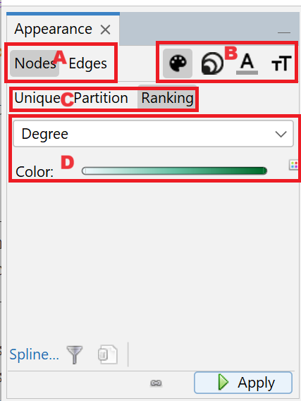
Figure: The "Appearance" subwindow to change node and edge (label) color and size
Task 2.3a: Set the node size proportional to a ranking based on degree (number of connections), and node color based on indegree (number of incoming connections). Your visualization may look something like the figure below. (For now, ignore the "Partition" tab; it will be discussed in Part 4: A real-world network visualization.)
Task 2.3b: Node size is proportional to the size of the Layout space; experimentally confirm how a larger value for the "Scaling" parameter of the "ForceAtlas 2" algorithm will require a larger minimal and maximal value for node size. Play with different node color schemes (through the icon to the right of the colored bar in the "Ranking" tab).

Figure: Stylized visualization of a random directed graph with 50 nodes
The label of a node (or edge) is a readable description of the node (or edge). In a social network it can be someone's real name, rather than a numeric ID. Label visibility can be enabled using the "Show Node Labels" button in the set of icons at the bottom of the Graph subwindow (button G in the figure below). One or more of the data attributes of the nodes are then shown as textual label; button Q allows one to set which attributes this pertains. By default, the "Label" node attribute is used, which in case of the random graph is equal to the ID of the node.
 Figure: Buttons at the bottom of the Graph pane
Icon A resets the viewport such that the entire network is visible; buttons B-D reset certain visual properties. Label G through Q adjust various meaningful aspects of the labels, such as their size, font and color, as well as provide the opportunity to adjust properties and visibility of the edges. Note: sometimes, edges become hard to see as nodes are colored, which can sometimes be counteracted with button I.
Task 2.4: Enable node labels, and play around with the various buttons A-P and observe what happens to the visualization.
Next, we will learn how to modify the network data underlying a Gephi visualization.
We turn to Gephi's second main window, being the Data laboratory. For a random graph, it should look like the figure below.
Here, the data behind the network can be inspected. On the top left, it is possible to switch between "Nodes" and "Edges"; which brings up the node list or the edge list in the data table below.
A node is always identified by a (typically numerical) Id. An edge is in turn defined by a Source and a Target, of which the values refer to the Id of a node.
 Figure: Gephi's Data laboratory, showing the edge list (so, after pressing "Edges" on the top left)
The Data laboratory can be used to manually change the data behind the graph, i.e., adding, removing and modifying the nodes, edges and their attributes. Adding nodes and edges can be done by using the respective buttons on top of the data table, and modifying one particular node or edge can be done by right clicking and selecting edit-option. Changes the the columns or column-wise modifications for all or multiple rows, can be effectuated using the buttons at the bottom of the data table.
Task 3.1: Create a new graph in which you represent your direct/close family members as nodes, and the blood connections between them as edges. Add a node attribute "Label" for their name, as well one for their "Age". You can also add an edge attribute of choice (for example, a binary attribute indicating whether the two family members physically live together). When your data is complete, visualize the graph in the "Overview" tab; be sure to enable labels and choose meaningful colors for the nodes and edges based on either network properties or attributes.
The node and edge lists of Gephi can also be filled by importing data from CSV files, or even (Excel) spreadsheets. For this, use the "Import spreadsheet" button, which invokes an import window. (Note that the same type of import window can be invoked when using the "File", "Open" menu button, and selecting a non-Gephi file that does have properties of a data file, i.e., is column-based.)
Along the way, you are asked to select the right data format. Here, "Edges table" and "Nodes table" are the edge list and node list formats most commonly used, with Id being the identifier column in the node list, and two columns Source and Target in the edge list.
The final screen asks whether the graph should be directed or undirected, and whether the data should be appended to the current workspace, or whether a new workspace should be made. The append-option can be used to merge multiple datasets based on the unique identifier Id of the nodes.
Task 3.2: Download the small-gephiready.tsv edge list file, and load it into Gephi via the Data laboratory. This .tsv file has tab-separated columns. Go back to the Overview screen and create a visually appealing visualization. The rest of the tutorial will also use this dataset.
Similar to importing, both the node and edge lists can also be exported for reuse in another tool using the "Export table" button. You can then reuse or amend this data, for example in Excel, or in a python pandas dataframe.
Now that we know how to manipulate the data behind a visualization, it's time to explore more advanced network analysis and visualization options in Gephi. We turn back to the Overview tab, and assume that the small-gephiready.tsv file has been loaded as an undirected graph. After visualizing this graph using the ForceAtlas2 algorithm with the scaling parameter set to 5.0, the screen should look something like below.
 Figure: Visualization of the small-gephiready.tsv network
Through the Statistics window, various properties of the network can be computed. After computation, so after pressing the button corresponding to the statistic, an overview window is produced showing some results. Typically the value or distribution of that statistic is shown (albeit in a suboptimal visual, missing for example logarithmic axes). But more importantly, in the node list, a column is added containing the value of that particular metric. Many of these metrics are known as centrality measures, that determine the importance of a node based on the structural position of that node in the network. This centrality value can in turn be used to adjust for example the color or size of a node (see Part 2: A first visualization of a network).
- Average Degree: computes the average degree of nodes, and adds the
Degreecolumn to the node list (and Indegree and Outdegree in case of directed graphs). - Avg. Weighted Degree: same as above, but then specific to weighted networks.
- Network Diameter: computes the radius and diameter (minimal and maximal shortest path length) values, as well as
Eccentricity,Closeness centrality,Harmonic closeness centralityandBetweenness centralityvalues for each node. - Graph Density, Avg Clustering Coefficient, Avg. Path Length: computes these metrics (one value for the graph as a whole).
- PageRank, HITS, Eigenvector centrality: computes these centrality measures, adding columns
PageRank,HITSandEigenvector centralityto the node list - Connected components: assigns to each node a
Component IDthat indicates which component (group of nodes connected by (paths of incident) edges) it belongs to. - Community detection: covered below.
Task 4.1: Compute Betweenness centrality and PageRank for the small-gephiready.tsv graph and in the visualization, set respectively node color and size proportional to these two measures. Observe their values in the Data laboratory, and determine the top five nodes based on each measure.
Apart from computing measures that say something about the nodes or the graph as a whole, we may also be interested in groups, i.e., clusters in the network, which in a network analysis context are called communities. Various algorithms for detecting these communities exist, and under the "Community detection" header, two of these algorithms can be found.
- Community detection (multiple algorithms): compute an integer value for each node that becomes a node attribute. For example, "Modularity", indicating to which community a node belongs based on an optimization process maximizing the number of intra-community links and minimizing the number of links between communities. A resolution parameter can be used to increase or decrease the number of communities found.
Task 4.2: Run Modularity and color (partition) the nodes based on their community (the Modularity Class attribute). The result should roughly look like the figure below.
 Figure: Visualization of the small-gephiready.tsv network, with node color based on community structure, and node size based on PageRank
The tab next to Statistics opens up a set of filters. These filters can be used to only display certain parts of the graph. You can select a filter and drag it to the "Queries" list below, to activate it. Some noteworthy filters include:
- Topology, Giant component: only show the largest connected component (does nothing in case the network consists of just one connected component, such as in our practice file).
- Attributes, Partition: only show nodes of which an attribute has a certain value.
- Attributes, Range: only show nodes of which an attribute is a certain range of values; for example setting a cut-off value for the degree, or based on centrality.
- Edges, Edge Weight: an often useful filter to, for a weighted network, only show the strongest links (handy when the graph is too dense to meaningfully visualize).
Note that filters can also be combined (which is not always intuitive).
Task 4.3: Use the filters to visualize one of the communities you found, and observe what happens to the Data laboratory as the filter is enabled.
You now have all the skills to visualize a network in a meaningful way, and time to export a picture-perfect version of it for reuse; for example in a presentation, report or a paper.
In the third Gephi tab, being Preview, it is possible to change final visual properties before exporting the visualization as crafted in the Overview tab. The "Refresh" button in the bottom right should be pressed to update the visualization. The visual you get may not look identical to what you see in the Overview tab. In particular, the option "Curved" of the edgges needs to be disabled.
After adjusting the desired properties of the Nodes, Node Labels, Edges and Edge Labels on the left, the button "Export: SVG/PDF/PNG" leads to a screen where the destination of the output file can be chosen. Be sure to choose a vector graphic format such as SVG, or, usually easiest, PDF. In this final window, the "Options" button on the bottom right.
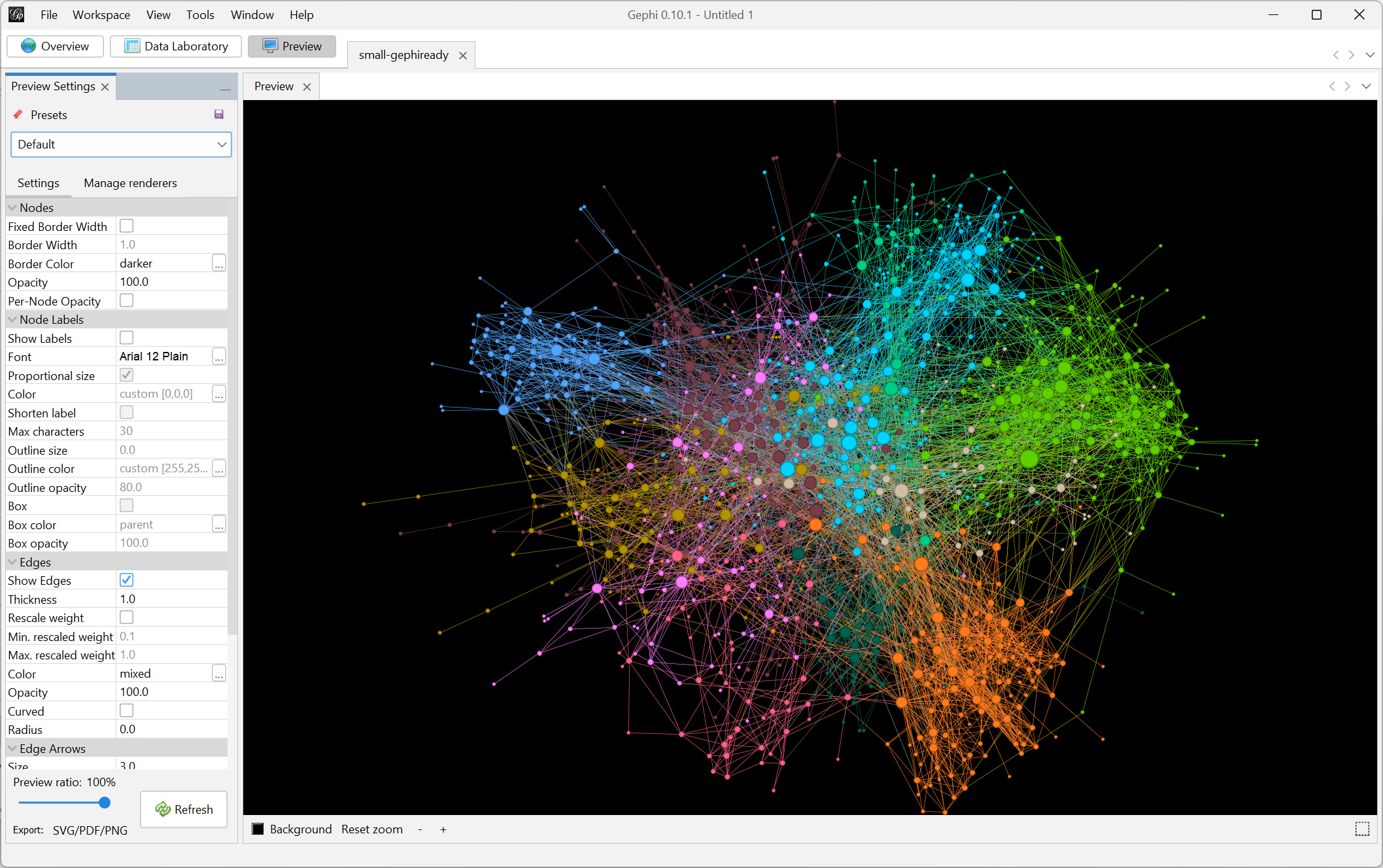 Figure: Gephi's Preview tab for exporting the visualization for reuse
Task 5: Export your visualization of the small-gephiready.tsv file into a rectangle-shaped vector graphic PDF, with a colored background if desired.
Based on the tutorial above, you will likely develop your own iterative process in which you import data, and then play with layout algorithms, filters and statistics, before exporting a finalized network visualization.
Many more things are possible with Gephi, often implemented through Gephi Plugins.
-
Weighted networks; although not covered in this tutorial, the "Weight" column of the edge list essentially facilitates this type of underlying network data.
-
Dynamic networks that change/evolve over time; see Gephi's documentation on dynamic networks
-
GeoLayout to visualize nodes at particular coordinates on the world map often used together with MapsOfCountries to show the outline of the world, a country or region.
-
MultimodeNetworksTransformationPlugin: a plugin for network projection, i.e., for modifying a network with multiple types of nodes (as defined by particular categorical node attributes), i.e., multipartitie networks, to unipartitate networks that can be meaningfully analyzed using Gephi.
-
The BoundingDiameters algorithm for quickly computing the exact diameter (longest shortest path length) of a network.
-
The Leiden Algorithm, a community detection algorithm similar to "Modularity" discussed above, but solving a number of bugs and generally attaining higher quality partitionings of the network.
Thank you for walking through this tutorial! I hope you enjoyed it.
See details on top on how to reference this tutorial. Feedback and suggestions are welcome (via Github "Issues"); also (and especially!) from students.