
The goal of this project is to develop a pipeline which is capable to detected the left and right ego lane pavement markings. The following chapters give a short insight into the camera calibration method, the image pre-processing pipeline and the lane detection pipeline. Finally the achieved results are discussed an demonstrated in a short video.
The goals / steps of this project are the following:
- Compute the camera calibration matrix and distortion coefficients given a set of chessboard images.
- Apply a distortion correction to raw images.
- Use color transforms, gradients, etc., to create a thresholded binary image.
- Apply a perspective transform to rectify binary image ("birds-eye view").
- Detect lane pixels and fit to find the lane boundary.
- Determine the curvature of the lane and vehicle position with respect to center.
- Warp the detected lane boundaries back onto the original image.
- Output visual display of the lane boundaries and numerical estimation of lane curvature and vehicle position.
The following list gives a short overview about all relevant files and its purpose.
- Calibration.py calibrates the camera based on a couple of chessboard images. The class determines the intrinsic and extrinsic calibration parameters.
- calib.dat stored extrinsic and intrinsic calibration results from Udacity's chessboard image set.
- CoreImageProcessing.py provides basic (core) image processing algorithms like gradient, gradient directions, magnitude, histogram calculation and threshold methods.
- LaneDetection.py detects the left and right ego lane pavement markings on an RGB image.
Before detection pavement markings in an image, the image has to be undistorted in order to detect a straight line as straight line. Without compensating the lense distortion a straight line might look like a curved one. To remove these effects, I implemented the Calibration.py class which handles all camera calibration tasks like extrinsic and intrinsic calibration based on chessboard images, saving/loading of calibration parameters and finally a method to undistort the image.
The camera can be calibrated by the following call. The calibration result will be stored in a pickled binary file (*.dat) which can be read out once by the Calibration class before the image processing pipeline.
python Calibration.py -c ./camera_cal -s calib.dat
The following lines shows the results of the calibration process. The rvecs and tvecs are not shown here.
Calibrated successfully based on 17/20 chessboards.

mtx:   [[  1.15396093e+03   0.00000000e+00   6.69705357e+02]
        [  0.00000000e+00   1.14802496e+03   3.85656234e+02]
        [  0.00000000e+00   0.00000000e+00   1.00000000e+00]]
dist:  [[ -2.41017956e-01  -5.30721173e-02  -1.15810355e-03  -1.28318856e-04 2.67125290e-02]]

Saved calibration data to calib.dat
Supported Console Parameters
python Calibration.py

  Camera Calibration

  optional arguments:
    -h, --help            show this help message and exit
    -c PATH, --calibrate PATH
                          Calibrates the camera with chessboard images in PATH.
    -s DAT_FILE, --save DAT_FILE
                          Save camera calibration to file to dat file
    -t DAT_FILE, --test-undistort DAT_FILE
                          Undistort test image with calibration dat file.
The code for the calibration step can be found in the method calibrate_with_chessboard_files(self, path, nb_corners) in the Calibration class.
First I prepare two arrays. The obj_points, which will be the (x, y, z) coordinates of the chessboard corners in world coordinates and the img_points representing the pixel position (x, y) of the detected chessboard corners in the image plane. To find the chessboard corners, I applied the OpenCV function cv2.findChessboardCorners(). The following image exemplifies the detected corners on a 9x6 chessboard.

Every time I successfully detect all chessboard corners (9x6) in the calibration image, the detected corners and the objp will be appended to the arrays. Finally, I use the cv2.calibrateCamera() function with the two array obj_points and img_points to determine the calibration (mtx) and distortion (dist) coefficients.
The undistort(self, image) method applies the determined coefficients by using the cv2.calibrateCamera() function to undistort the camera image. The result is shown in the images below.
As you can see in the chessboard images the lens distortion is getting worse especially in the image border areas. This effect can also be observed in the image with the red car below. In the undistorted image it looks like the red car is located closer to the ego vehicle compared to the distorted image. The same effect can be observed on the dashed line markings.

The whole pipeline is implemented and controlled by the method detect_ego_lane(self, image) in the LaneDetection.py file. The pipeline consists of the six steps as described below.
- Image pre-processing to undistort the image and to calculate a thresholded binary image representing the lane marking boundaries
- Warping of the binary image into a "birds-eye-view"
- Identification of left and right lane-line points
- Polynomial fit through the identified lane-line points
- Calculation of the curve radius and the vehicle position within the ego lane
- Sanity checks to avoid outliers
The task of the image pre-processing pipeline is to provide a binary image in which pavement marker candidates are represented by an "1" and non relevant areas by a "0". The graph below describes all steps performed in the preprocess_image(self, image) method.

Color Spaces and Channel Thresholding
The pre-processing pipeline undistorts the RGB input image, extracts the red and blue channels from the RGB color space and the lightness and saturation channels from the HLS color space. The red channel is used to identify white and yellow markings. The blue channel almost does not see yellow markings but strongly supports the white marker extraction. The saturation channel returns all areas with saturated colors. Under normal conditions these are mainly yellow and white colored markings.
Afterwards each channel has been thresholded to reduce non lane marking areas to a minimum. For red I used a threshold of 190-255, for blue 185-255, for lightness 135-255 and for the saturation 100-255. The results of this step are depicted in the image below.

x-/y-Gradients and Magnitude Thresholding
In order to increase the detection range I calculate the x- and y-gradients with a sobel kernel size of 13 and the magnitude for the red and blue channels. The images below exemplifies the results of this processing step. One interesting aspect can be seen in the blue channel images. The blue channel almost delivers no line candidates in the color threshold image for yellow markers but the x-gradient clearly marks the yellow solid line.

Handling of cast shadows
In cast shadow scenarios the red and blue channels are not sufficient for a stable lane marker detection. They either deliver almost nothing or just noise. The saturation channel looks quite noisy because it highlights the yellow lane line and all cast shadow areas. In contrast, the lightness channel highlights all bright areas, thus the shadow areas are suppressed. Finally, I combined the lightness and saturation binary images with a bitwise AND operation. As a result the yellow solid line gets clearly visible in the binary image (see figure below).

Adaptive Red Color Channel Thresholding
To find the best thresholds for the red channel was a bit tricky. On bright concrete the channel tends to "bleed out" (as depicted in the right image in the figure below). If I increase the threshold it works well on bright concrete but delivers less information under normal conditions. Therefore, I introduced an adaptive threshold for the red color channel. The algorithm calculates the percentage of the activations ("1") in the roadway area of the thresholded binary image. Base on the result I chose between three threshold sets as explained in the table below.
| Threshold | Percentage | Range | Description |
|---|---|---|---|
| T0 | 0.032 | (190, 255) | Useful for yellow lines on dark surfaces |
| T1 | 0.04 | (210, 255) | Suppress bleeding effects on bright concrete |
| T2 | 0.1 | (230, 255) | Extreme suppression of bleeding on bright concrete |

Combination of Binary Threshold Images
The last step in the image pre-processing method is the combination of all binary images. The image below explains all applied bitwise AND and OR operations step by step. The image depicted in the bottom row shows the output of the pre-processing step.

The perpective transfomation of the image is implemented in the warp(self, image, src_pts, dst_pts, dst_img_size=None) method in my CoreImageProcessing class. The method takes an image (image), the source points (src_pts), the destination points (dst_pts) and optional a new destination image size (dst_img_size). I manually chose the source points in the image (marked left and right lane line in the near and far range) and hardcoded these points in the following manner.
warp_img_height = 720
warp_img_width = 1280
warp_src_pts = np.float32([[193, warp_img_height],
                           [1117, warp_img_height],
                           [686, 450],
                           [594, 450]])
warp_dst_pts = np.float32([[300, warp_img_height],
                           [977, warp_img_height],
                           [977, 0],
                           [300, 0]])
I verified that my perspective transform was working as expected by drawing the src_pts and dst_pts points onto a test image and its warped counterpart to verify that the lines appear parallel in the warped image.

My lane-line search algorithm consists of two different types of algorithms. In case no valid lane-lines have been detected, I apply a sliding window histogram search on the warped binary image. The algorithm calculates a histogram on the lower part of the image. The two highest peaks in the histogram marks the first two search areas for the sliding window approach which detects the full lane-lines.
Because this procedure is very computational intensive, I apply the histogram based search for the initial lane-line detection only. Once the lane-lines are detected in the previous frame, a less computational intensive search algorithm is applied. This algorithm assumes that the new lane-lines look similar to that ones in the previous frame. Thus algorithm searches +/- 100 pixels around the previous polynomial fit for lane-line pixels.

In the next step, I fit two independent second order polynomials through the left and right lane line pixels. The polynomial is described by the following formula:
f(y) = A * y^2 + B * y + C
To calculate the curve radius and the ego-vehicle position we first need to know, how to convert pixel coordinates into world coordinates. The US regulations require a minimum lane width of 12 feet (3.7m) and dashed lane lines with a length of 10 feet (3.0 m). In the birds-eye-view I measured 652 pixels in average for the ego lane width on a straight road and 80 pixels in average for a dashed marker segment. Furthermore, I assumed that the camera position is mounted exactly in the center of the vehicle's windscreen.
xm_per_pix = 3.7 / 652      # meters per pixel in x dimension (lane width in US = 3.7 m)
ym_per_pix = 3.0 / 80       # meters per pixel in y dimension (dashed marker length in US = 3.0 m)
cam_pos_x = 1280 / 2.       # camera x-position in pixel (center of image)
For the curve radius I applied the formula as stated in the code below. The detailed derivation can be found in this Tutorial. First I convert the pixel coordinates into world coordinates and calculate the left and right polynomial fits on these coordinates. Afterwards I use the curve radius formula to calculate the radius at the nearest point to the ego vehicle (yr = np.max(line_fit_y)).
def calc_curve_radius(self, x, y, yr, degree=2,):
  """ Calculated the curve radius in world space)

  :param x:         x-values (array of points) in image space.
  :param y:         y-values (array of points) in image space.
  :param yr:        y-position at which the curve radius shall be calculated in image space.
  :param degree:    Degree of polynomial. Default = second order polynomial

  :return: Returns the curve radius in meters (world space)
  """

  line_fit_w = self.fit_line(x, y, degree=2, coordinate_space='world')
  return ((1 + (2 * line_fit_w[0] * yr * self.ym_per_pix + line_fit_w[1])**2)**1.5) / np.absolute(2 * line_fit_w[0])
The whole code can be found in the LaneDetection.py (line 451-468) file. In adition to the curve radius I also calculate the lane width (lane_width), the vehicle's offset from the center line (d_offset_center) and the distance to left (d_left) and right (d_right) lane markings as stated below.
# calculate lane width, center offset and distance to left/right ego lane boundary
# world coordinate system: x forwards, y left
lane_width = (line_fit_right_x[-1] - line_fit_left_x[-1]) * self.xm_per_pix
lane_center = (line_fit_right_x[-1] + line_fit_left_x[-1]) / 2.
d_offset_center = (self.cam_pos_x - lane_center) * self.xm_per_pix
d_left = (self.cam_pos_x - line_fit_left_x[-1]) * self.xm_per_pix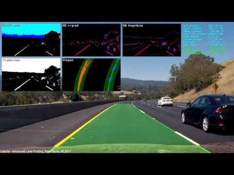
d_right = (self.cam_pos_x - line_fit_right_x[-1]) * self.xm_per_pixThe image below shows the detect_ego_lane() input image with all activated debug overlays. In the top left the Red, Lightness&Saturation and Blue color threshold image is displayed, followed by the Red and Blue channel x-gradient threshold image, and the Red and Blue channel magnitude threshold image. In the top right of the overlay I display the curve radius, the vehicle offset from center line and internal status information like chosen red channel thresholds, sanity checks, etc. In the second row the combined binary image and the warped binary image (birds-eye-view) with identified left and right lane line pixels are illustrated.

Video on GitHub
YouTube Video
The color thresholds are very sensitive to environmental conditions like sun, rain, day and night. The currently chosen thresholds won't work e.g. during night. One solution could be a measurement method to calculate the optimal thresholds online (similar to the method I implemented for the red channel).
Furthermore, I'd like to implement a ego lane tracker to stabilize the detected lane-lines. Unfortunately, the Udacity dataset does not include any vehicle odometry data like speed, yaw rate, etc. Therefore, I just implemented an simple filter to stabilize the lane-lines between two consecutive frames.
Finally, the lane-line pixel identification is not the optimal solution. Especially on the challenge videos this method frequently produces false positives. To solve this issue you either need more complex algorithms analyzing the lane marker characteristics followed by a couple of sanity checks or completely new methods which has some knowledge about the semantics of the individual pixels. First approaches with CNNs are described e.g in this paper "An Empirical Evaluation of Deep Learning on Highway Driving" from the Stanford University.