Computation of integration based prediction bands
Here, a basic introduction to the integration-based computation of prediction bands (PBs) on the model dynamics will be given. The example in /Examples/ABC_toyModel was added in the revision of 07/22/2015.
The integration framework is located in the folder /PPL.
It allows to compute prediction bands on the whole time-course of model dynamics of the model components (internal states) as well as for the observations. In addition, new observations like ratios or sums of the internal states or observations can be added to the model and their prediction band can be calculated.
At the beginning, a validation profile likelihood is computed (see Likelihood based observability analysis and confidence intervals for predictions of dynamic models. ). Thereof, the auxiliary data point and parameter set to a specified confidence level is taken as starting point for the integration.
Based on the penalized likelihood-function, a system of ODEs is obtained and executed to establish the prediction band.
Note that the resulting integrated prediction band does not specify pure prediction uncertainty, but includes the unceratinty of the auxiliary data point, as briefly explained in the article Estimating Prediction Uncertainty. Since the computation of actual prediction bands is not supported by the integration method, they are obtained by calculation of prediction profiles at several time points. If such an approach is chosen, refer to the article Discrete Sampling of True Prediction Bands.
The integration of prediction bands based on validation profiles is now demonstrated on an example. To run the ABC toy model in the Examples folder, at first the D2D framework is initialised and the model and data is loaded, followed by a compilation of them.
arInit

arLoadModel('ABC_model');
arLoadData('ABC_data_BCobs');

arCompileAll();
Further, the standard deviation of 0.1 which was taken for the data simulation is fixed for the optimisation procedure, which is then performed:
ar.config.fiterrors = -1;
arSetPars('sd_B_au',[],2);
arSetPars('sd_C_au',[],2);

arFit();
Subsequently, to obtain the prediction bands on all three states A, B and C, the function arPPL is used.
It takes the desired model as first input and the condition or data, dependent on the fifth flag (takeY).
Also, the desired internal states for which PBs should be computed have to be stated as third input (in this case 1:3).
In addition, a vector t can be added for which the complete validation profile should be calculated. In the final plot, black stars indicate the alpha thresholds of the hereby obtained prediction intervals.
The first time point stated will be used as starting point of the integration.
The arPPL statement in the Setup.m of the ABC toy example is given by
PPL_options('integrate',true)
arPPL(1,1,1:3,linspace(0,100,11),1);
where integration is turned on in the options before the PPL script is executed.
The integrated prediction bands can be plotted via
arPlot2
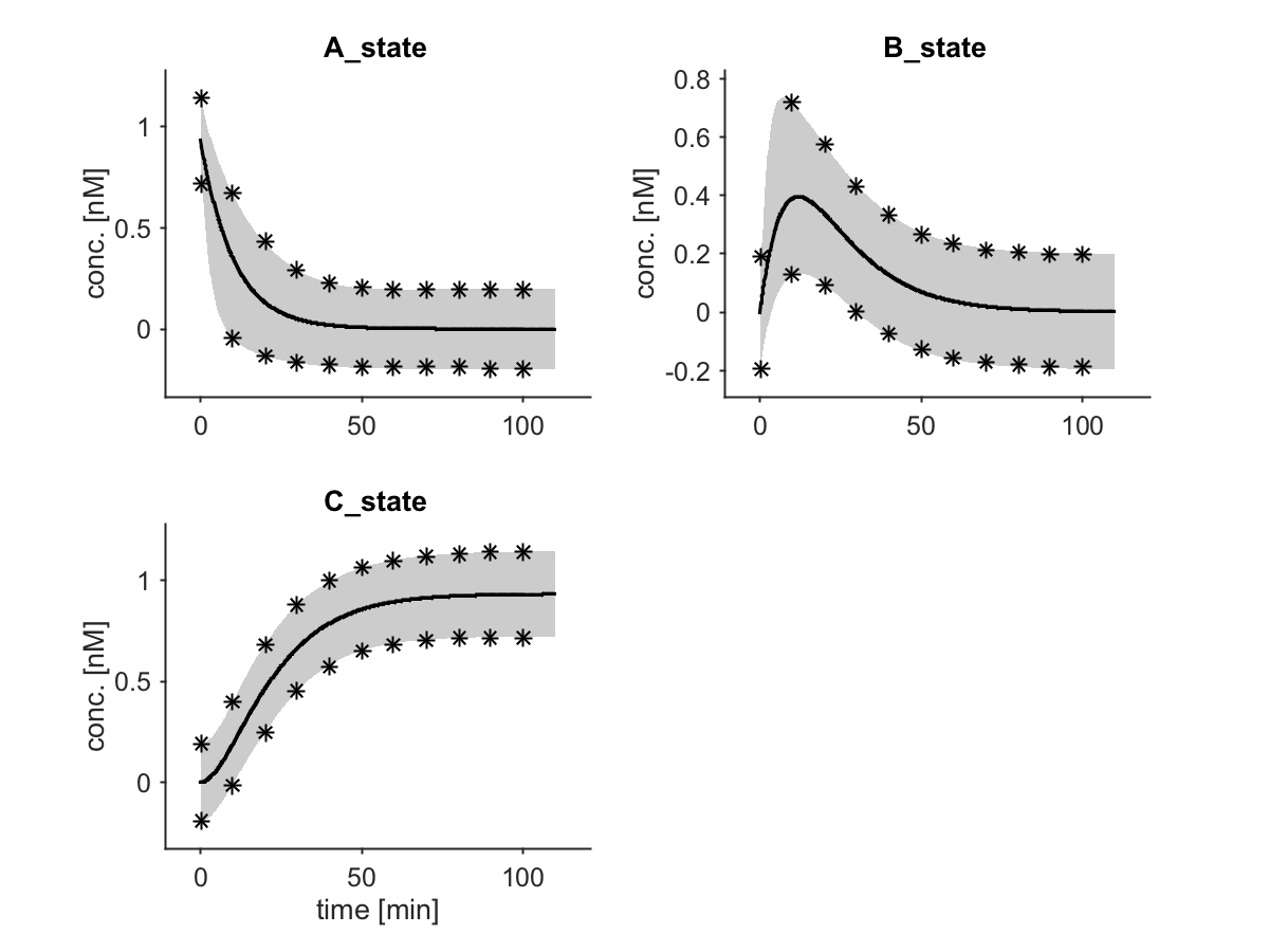
The plot then shows the data points as dots, the best fit as solid line and the PBs as shaded area, together with the thresholds of the confidence intervals calculated via validation profile likelihood for the stated time points:
Prediction bands in a Systems Biology application can be computed for the Swameye example at /Examples/Swameye_PNAS2003 (by commenting out the arPPL command in its Setup.m).