Skip to content
evazlimen edited this page Sep 23, 2023 · 1 revision

3D Brio and Wu MHD Shocktube

Similar to the Sod shock test but includes magnetic fields. Illustrates the ability of a code to resolve shocks and contact discontinuities over a narrow region. Parameters from Brio & Wu (1988). For more testing information see MHD Riemann Problems. The test consists of two constant states (on left pressure and density are equal to 1; on right they are equal to 0.1 and 0.128, respectively) separated by a discontinuity at 0.5. The left side has a magnetic field of 0.75 $\hat{x}$ + 1 $\hat{y}$ while the right side has a magnetic field of 0.75 $\hat{x}$ - 1 $\hat{y}$. Gamma is set to 2.0. This test is performed with the mhd build (cholla/builds/make.type.mhd).

Parameter file: (cholla/examples/3D/Brio_and_Wu.txt)

#
# Parameter File for 3D Brio & Wu MHD shock tube
# Citation: Brio & Wu 1988 "An Upwind Differencing Scheme for the Equations of
# Ideal Magnetohydrodynamics"
#

################################################
# number of grid cells in the x dimension
nx=256
# number of grid cells in the y dimension
ny=256
# number of grid cells in the z dimension
nz=256
# final output time
tout=0.1
# time interval for output
outstep=0.1
# name of initial conditions
init=Riemann

# domain properties
xmin=0.0
ymin=0.0
zmin=0.0
xlen=1.0
ylen=1.0
zlen=1.0

# type of boundary conditions
xl_bcnd=3
xu_bcnd=3
yl_bcnd=3
yu_bcnd=3
zl_bcnd=3
zu_bcnd=3

# path to output directory
outdir=./

#################################################
# Parameters for 1D Riemann problems
# density of left state
rho_l=1.0
# velocity of left state
vx_l=0
vy_l=0
vz_l=0
# pressure of left state
P_l=1.0
# Magnetic field of the left state
Bx_l=0.75
By_l=1.0
Bz_l=0.0

# density of right state
rho_r=0.128
# velocity of right state
vx_r=0
vy_r=0
vz_r=0
# pressure of right state
P_r=0.1
# Magnetic field of the right state
Bx_r=0.75
By_r=-1.0
Bz_r=0.0

# location of initial discontinuity
diaph=0.5
# value of gamma
gamma=2.0

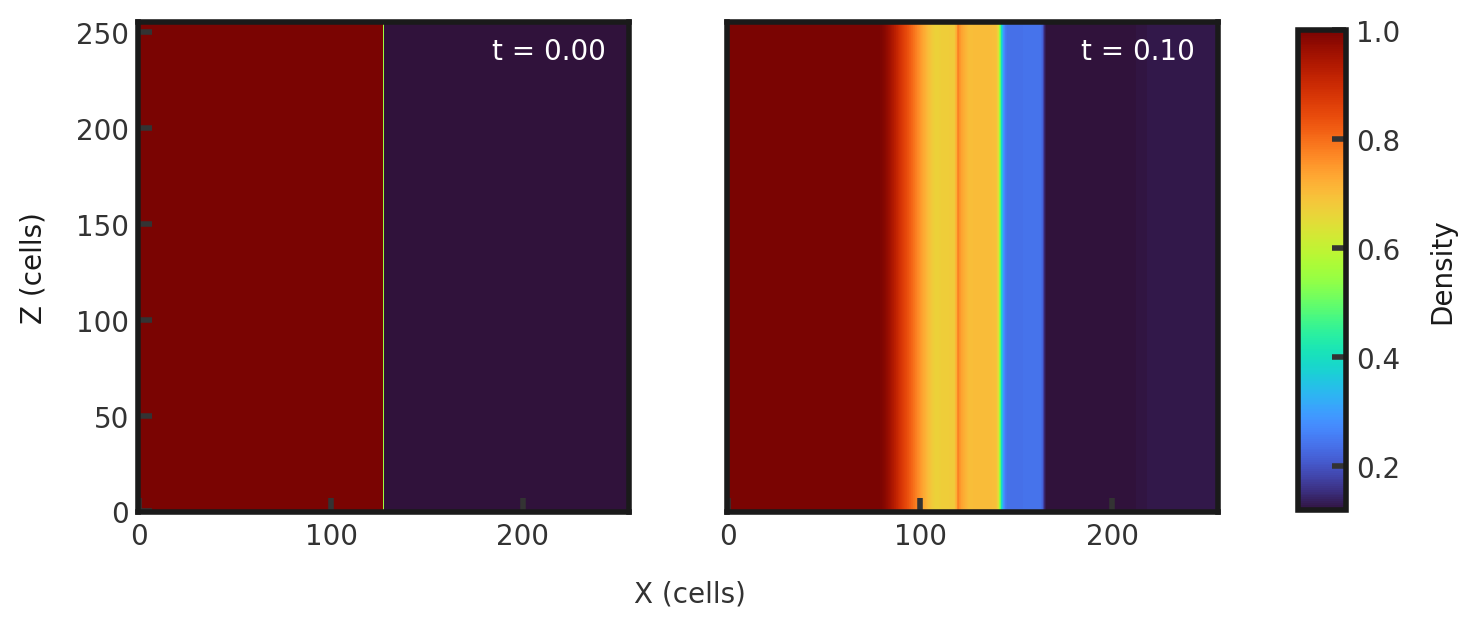
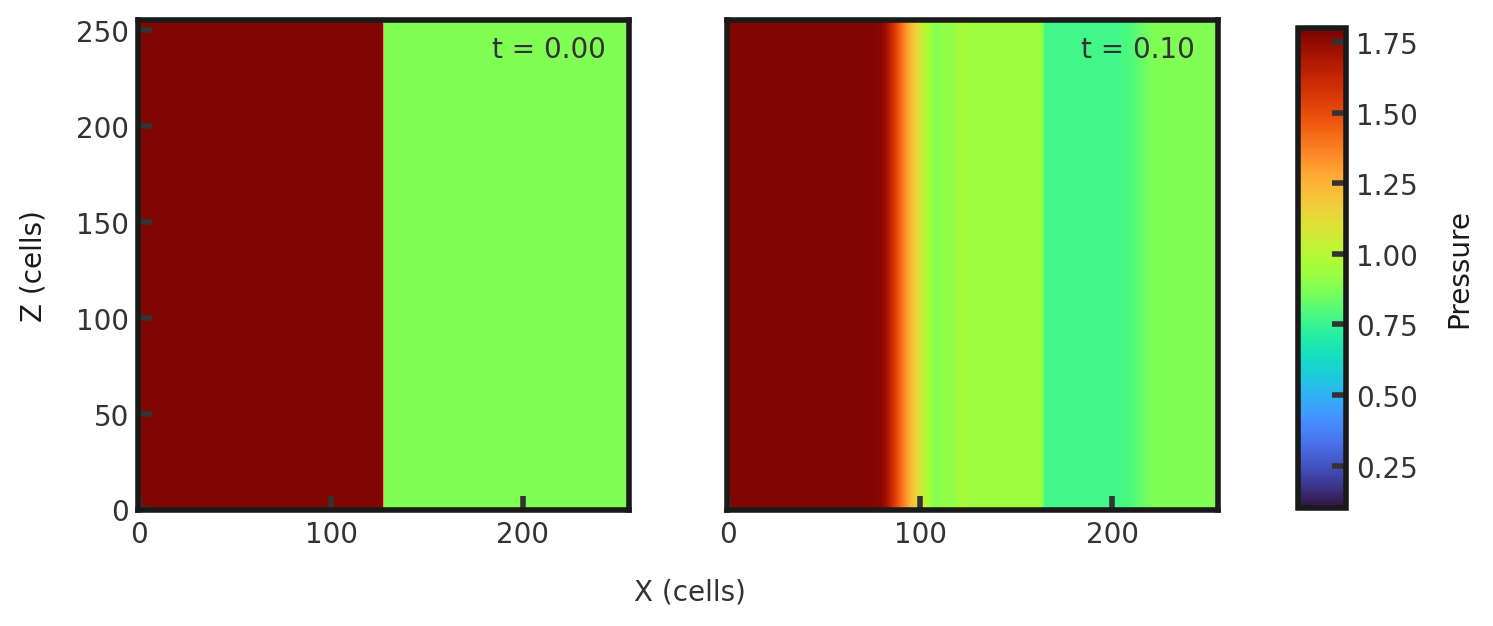
Upon completion, you should obtain two output files. The initial and final densities and total pressures (in code units) of a slice along the y-midplane is shown below. Examples of how to plot projections and slices can be found in cholla/python_scripts/Projection_Slice_Tutorial.ipynb.

Two 2D histograms side by side, showing density of cells in the z direction vs cells in x direction. The leftmost is the initial density plot with a constant density of 1 throughout all 256 z cells between x-cells 0 through 128 and a constant density of 0.128 between x cells 128 through 256. The rightmost plot is the final density plot at t = 0.10 with a nonconstant density in x and constant density in z. A density of 1 begins decreasing around x = 80 cells to around 0.7 but briefly and abruptly jumps to 0.8 around x = 125 cells. It is then constant around 0.7 until x = 150 cells where it jumps to 0.3 and remains constant until x = 175 where it jumps to 0.1. Two 2D histograms side by side, showing pressure of cells in the z direction vs cells in x direction. The leftmost is the initial pressure plot with a constant pressure of 1.8 throughout all 256 z cells between x-cells 0 through 128 and a constant pressure of 0.8 between x cells 128 through 256. The rightmost plot is the final pressure plot at t = 0.10 with a nonconstant pressure in x and constant pressure in z. A pressure of 1.8 begins decreasing around x = 80 cells to around 1.0 but briefly and abruptly jumps to 1.1 around x = 125 cells. It is then constant around 1.0 until x = 150 cells where it jumps to 0.8 and remains constant until x = 200 where it smoothly increases to 1.0.

A skewer in x along y and z midplanes yields the 1-dimension solution at t = 0.10:
A set of 6 scatter plots. Top row: Density vs position and Pressure vs position. Second row: x velocity vs position and y velocity vs position. Third row: magnetic field in the y direction vs position and energy vs position. The density plot shows a value of 1 begin decreasing around x = 80 cells to around 0.7 but briefly and abruptly jumps to 0.8 around x = 125 cells. It is then constant around 0.7 until x = 150 cells where it jumps to 0.3 and remains constant until x = 175 where it jumps to 0.1. The pressure plot shows a pressure of 1.8 begin decreasing around x = 80 cells to around 1.0. It briefly and abruptly jumps to 1.1 around x = 125 cells. It is then constant around 1.0 until x = 150 cells where it jumps to 0.8 and remains constant until x = 200 where it smoothly increases to 1.0. The x velocity plot shows a velocity of zero smoothly increase to 0.1 between x = 80 and 100 cells. It has a deo to 0.5 at x = 120 cells and then is constant until x = 175 cells. It then drops discontinuously to -0.2 and increases again to 0.0 between x = 200 and 210 cells. The y velocity plot shows a value of zero until x = 80 cels, where it decreases to -0.25 by x = 100 cells. It jumps down to -1.5 at x = 125 cells and jumps back up to -0.25 at x = 160 cells. It gradually increases to 0.0 between x = 200 and 220 cells. The y magnetic field plot shows a value of 1.0 until x = 80, ,where it decreases to a value of 0.5 by x = 100. It drops to -0.5 at x = 110 and drops agin to -1.0 at x = 175. It decreases from -1.0 to -1.1 between x = 200 and 205 cells. The energy plot shows a value of 1.75 until x = 80 cells, where it smoothly decreases to 1.0 at x = 100 cells. It jumps to 1.8 at x = 125 cells and drops to 1.25 at x = 150 cells. It drops again to 0.5 at x = 170 cells. It gradually increases to 0.6 between x = 200 and 220 cells
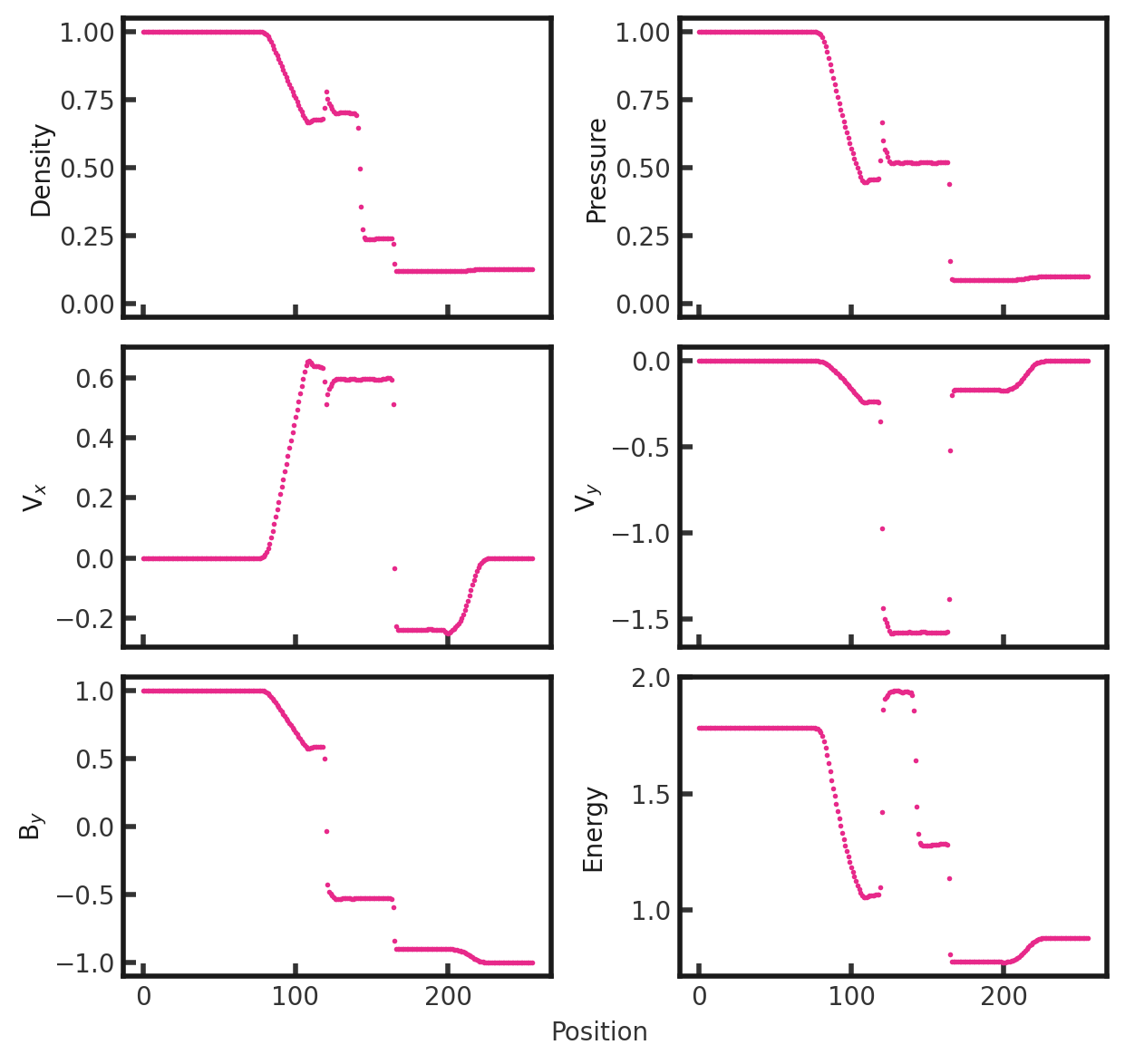
From left to right, we see a fast rarefaction followed by a compound wave, contact discontinuity, slow shock, and a final fast rarefaction.
We can compare to the original solution (Brio & Wu 1988):

Clone this wiki locally