Implemented PCA from scratch and performed dimensionality reduction over the datasets to improve the algorithm results
Dataset Description
The dataset contains the gene expression values for 20,531 genes across 800 cancer samples. Additionally, a CSV file called ’labels.csv’ indicates the type of cancer for each of the 800 data points. This data has been obtained from the TCGA project. The purpose of dataset can be to perform various analyses related to cancer biology, such as identifying biomarkers for different types of cancer,etc. This dataset can be used by researchers to develop predictive models to identify patients who may be at a higher risk of developing certain types of cancer.
Algorithm PCA Algorithm This part is provided to help you implement Principal Component Analysis. 1: ALGORITHM PCA 2: INPUT ∆: n × m data matrix of rank r, d: the number of new dimensions where d ≤ r. 3: OUTPUT ˆ∆: d dimensional representation of ∆. 4: %% mean centering - ∆ is the centered data matrix. 5: %% I denotes n × n identity matrix, e = (1, ..., 1) ∈ Rn. 6: ˜∆ ← (I − e.e^T/n) ∆ 7: %% Compute the SVD of ˜∆. σ1 ≥ ... ≥ σr > 0 are the strictly positive singular values of ˜∆. 8: %% u1, ..., ur and v1, ..., vr are the corresponding left and right singular vectors respectively. 9: ˜∆ ← P ri=1 σiuivit 10: ˆ∆ [σ1u1|...|σdud] = [δˆt1
...
δˆtn]
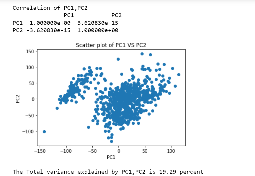
Experiments Perform PCA over the RNA-Seq data set and make a scatter plot of PC1 and PC2 (the first two principal components). Are PC1 and PC2 linearly correlated? How much of the variance can be explained by PC1 and PC2?
Have performed PCA on the RNA dataset. Please find the the scatter plot below. The points in the scatter plot are randomly spread out. There is no pattern in the scatter plot for PC1 and PC2, depicting no such relationship. This is confirmed by the correlation matrix plotted below. The value is −3.62 ∗ 10−15, very small, showing a very weak correlation among the first two Principal Components. Hence, PC1 and PC2 are not correlated. The total variance explained by PC1 and PC2 is 19.29 percent
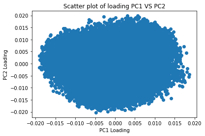
Loadings in PCA
Loadings in PCA indicate the correlation between original variables and principal components. They show the relationship strength and direction. Each principal component is a linear combination of original variables, with loadings indicating their relative importance. The first principal component accounts for the most variation and each successive component accounts for remaining variation. Loadings of the first component help to identify variables contributing most to data variation. They also help detect multicollinearity issues, where highly correlated variables may have similar loadings. Removing variables may be necessary to prevent over- representation. Loadings provide insight into the relationship between original variables and principal components and help interpret data.Here the scatter plot of PC1 and PC2 is shown in the figure below. Contribution of every variable to the formation of PCA is ranging from -0.02 to 0.02. The values seems randomly spread out forming a cluster and even the values are 0, showing no contribution. There are variables which are not contributing to the Principal components.
Performing Kmeans and hierarchical clustering on raw data and PCA data to check on the advantages of dimensionality reduction
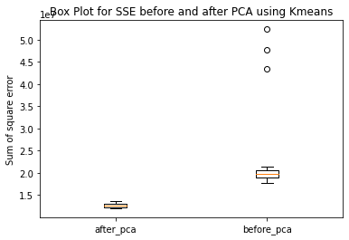
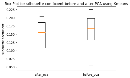
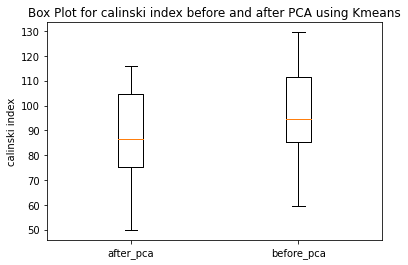
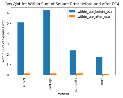
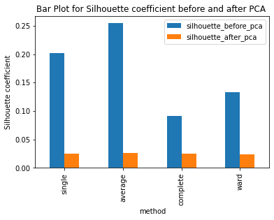
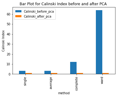
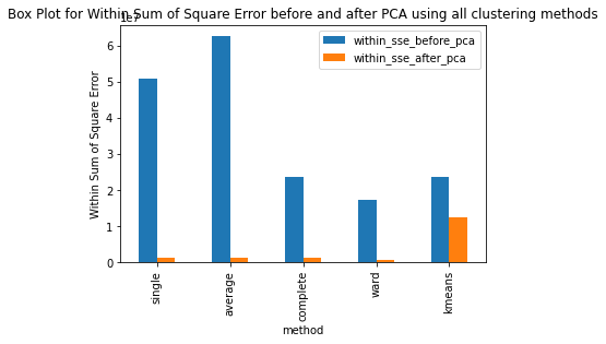
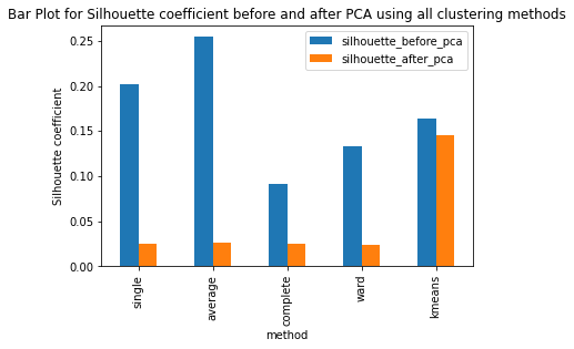
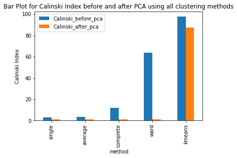
Have ran the kmeans clustering algorithm on the actual dataset for k=5 i.e number of clusters=5. Also ran 3 different hierarchical clustering algorithms on the actual dataset where the method for heirarchical clustering includes: ’single’,’average’,’complete’,’ward’. These methods are used to determine the distance between clusters based on the distances between their individual members. Single linkage: calculates the distance between two clusters based on the shortest distance between any two points in the clusters. Average linkage: calculates the distance between two clusters based on the average distance between all pairs of points in the clusters. Complete linkage: calculates the distance between two clusters based on the maximum distance between any two points in the clusters. Ward linkage: calculates the distance between two clusters based on the increase in the sum of squares that results when the two clusters are merged. Each of these methods has its own strengths and weaknesses and the choice of method will depend on the specific characteristics of the data being analyzed and the objectives of the analysis. For example, single linkage is sensitive to noise and outliers, while complete linkage can produce clusters of uneven sizes. Ward linkage tends to produce compact, spherical clusters and is often used when the goal is to minimize the variance within clusters. The different cluster validity techniques that are performed includes: The silhouette coefficient , Calinski�Harabasz index, and within sum of squares (WSS) are all appropriate techniques for evaluating the quality of clustering results. These indices are classified as internal ,relative and external indices.The silhouette index measures how well each data point fits into its assigned cluster compared to other clusters, the Calinski�Harabasz index measures the ratio of the between-cluster variance to the within-cluster variance, and the WSS measures the sum of squared distances between each data point and the centroid of its assigned cluster. These indices can be used together to get a comprehensive evaluation of clustering results. Have applied these validation techniques on the clusters formed after performing kmeans clustering and hierarchical clustering on the raw datset. The results of which are stored in dataframe. Perfomed PCA over the dataset to capture 99.99 variance, 724 principal components were generated. Applied kmeans clustering and hierarchical clustering on the reduced dataset (PCA) dataset and stored the results. From the graphs below it can be seen that: For kmeans clustering: The median within sum of square error after PCA is much less than that of the median within sum of square error after PCA. The median silhouette coefficient and Calinski index is also less for the data after PCA as compared to that of data before applying PCA (raw datset) For hierarchical clustering: The bar length of within sum of square error before performing PCA is much higher than the bar length of within sum of square error after applying PCA for all types of clustering. Also, the silhouette coefficient and Calinski index shows similar results of after and before PCA. Comparing all clustering algorithms: It can be seen from the graph of within sum of square error that the bar length of average method of hier�archical clustering is the highest before PCA and that of ward is the smallest. So ward method performed well before applying PCA. After applying PCA, the ward has the smallest error as compared to kmeans and other hierarchical clustering methods.So for the given dataset, Ward can be used as the technique to perform clustering, considering within sum of square error as metric. The silhouette coefficient for complete method is minimum when compared with that of other methods for both the dataset (before and after PCA). The calinski index is maximum for Kmeans clustering and miminum for clustering using single linkage method. Based on different validation techniques: Ward performed best when the within sum of square error validation was used. Complete linkage outper�formed when silhouette coefficient was used. Similarly, kmeans performed well using calinski index. Hence, it depends upon usecase and the given problem statement, to select a particular validation technique. Each has its pros and cons. To summarise, Clustering did improve after performing the PCA. THe error rates reduced.
Please refer the pdf file for series of steps and their output. Codes are available in the code folder for reference