Dataset The dataset contains information on patients with diabetes who were admitted to 130 hospitals in the United States between 1999 and 2008. The primary purpose of the dataset is to explore features that affect readmission rates for diabetic patients.The dataset can be used for various purposes, including exploring the relationship between various features like patient condition,labtest,medications and readmission rates, developing predictive models for readmission, and evaluating the quality of care provided by hospitals. The dataset can be used to identify the relationship between various parameters and can be used by Doctors, researchers to identify the mistakes or areas of improvements or what better could have been done , so that patient is not readmitted. Also, identify some pattern or cluster in the data given all the features or identify the main features affecting the readmission. The different data types that the dataset includes are integer and object data. The dataset’s features include patient demographics, admission type and source, diagnosis and procedure codes, lab tests, medications, length of stay,etc. The target variable is whether or not the patient was readmitted to the hospital within 30 days of discharge. Overall there are 101766 entries of data and 50 features/columns including the target variable.
Exploratory Data Analysis
Handling Missing Data There are no null entries as such in data. But some of the columns contains ? Replacing question mark with NAN. After doing that we can see the results and now this missing data needs to be handled. ′race′,′ weight′,′ payercode′,′ medicalspecialty′,′ diag1′ ,′ diag′2,′ diag′3 Columns contains null data. Dropping the columns where the count of null data is almost around 50 percent as they dont provide significant information.
Creating Histograms The histogram plot of the age feature suggests that the data is skewed towards higher age, while the histogram plot of the num lab procedures feature suggests that the data is skewed and bimodal. Furthermore, the histogram plot of the num medication feature indicates that the data is normally distributed and right-tailed.
Scatterplots The scatter plot of time in hospital and num medications shows a positive relationship between the two variables, which is also supported by the correlation matrix. The scatter plot also suggests that the readmitted variable does not have a strong relationship with either variable. Similarly, the scatter plot of num medications and num lab procedures shows a weak positive relationship between the two variables, which is also supported by the correlation matrix. The scatter plot also suggests that the readmitted variable does not have a strong relationship with either variable.
Implementation
Initialization of Gaussians
GMM (Gaussian Mixture Model) is a paramteric technique. The model is trained using the Expectation�Maximization (EM) algorithm. Before the expectation steps, there are certain assumptions about the data and initializations done, before the start of the actual algorithm. The main assumption is that for all the features, the data is distributed normally and then we use soft clustering to assign each data point to a cluster. The goal of GMM is to estimate the parameters of the underlying mixture model that best fit the observed data. The different vectors initialized are as follows:
- Mean Vector- The mean vector is initialized by randomly selecting the k data points from the data, considering them as the centroids coordinate. Here k is the number of clusters.
- Covariance Vector- The covariance vector is initially initialized by creating an identity matrix of size features* features. The vector contains k number of identity matrices where k is the number of clusters.
- Weight Vector- The weight vector is the weights of each cluster and initially all the clusters have same weight of 1/k where k is number of clusters. So the vector contains k weights each with a value of 1/k.
Maintaining k Gaussians
The EM algorithm keeps on switching between an Expectation step and a Maximization step. In the Expectation step, the algorithm estimates the probability that each data point belongs to each component. In the Maximization step, the algorithm updates the parameters of the model to maximize the likelihood of the observed data given the estimated component probabilities. The GMM is a soft clustering method i.e the data point is not rigidly assigned to each cluster, instead, we have a posterior probability vector that stores the likelihood of each point going into a cluster. Hence k clusters are maintained at each iteration. For a data point, the maximum probability for going into a cluster as per the posterior probability calculation is selected. After every iteration, the weights and mean vectors for each cluster are updated.
Deciding Ties
Here we maintain the posterior probability matrix for each data point and at every iteration. In case the probability of assigning a datapoint to cluster is same, I have used random selection , this means that in case of a tie between selecting a cluster, any conflicting cluster can be selected all having equal probability of getting selected.
Stopping Criteria
As per the algorithm provided, I have implemented a similar logic. When the mean vector is updated and the euclidean difference between the current centroid and the previous centroid is less than a particular threshold, in that case, the algorithm converges, and we get the final centroid coordinates, weight vector, probabilities, etc.
Comparision of Kmeans algorithm with GMM (EM) algorithm
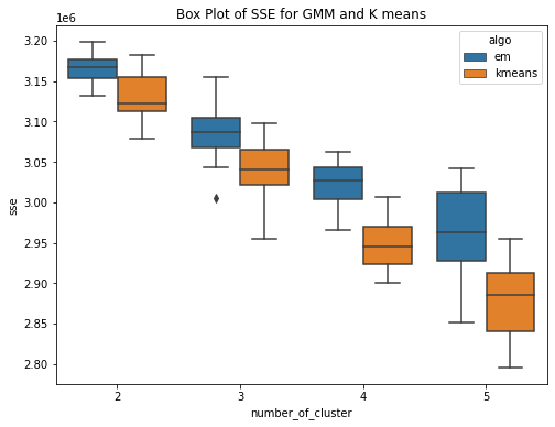
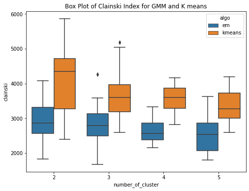
The GMM (EM) algorithm and K-means algorithm is ran over the diabetes dataset 20 times each for clusters ranging from 2 to 5.Have used within sum of square error and Calinski-Harabasz score to evaluate the clustering techniques. Within Sum of Squares (WSS), which calculates the total sum of distances between each point in a cluster and its centroid. Calinski-Harabasz score (CHS), which evaluates the quality of the clustering solution by comparing the separation between clusters to the dispersion within clusters. From the box plots, it can be seen that the median within the sum of square error for k means is less than the median within sse of EM. This means for the given dataset, K means have performed better or the clusters are well separated and the within-cluster the data points are very close to the centroid. Whereas for GMM, it has higher sse, one of the reasons could be the clusters formed are overlapping and this may lead to higher error. This can be confirmed by the Calinski Harabasz score (CHS). The median CHS score for kmeans is higher than that of the GMM for all the cluster, showing the clusters formed by Kmeans are well seperated. We can use other techniques to perform the validity and this highly depends upon the requirements and use case.
Performing PCA over the dataset and then comparing Kmeans algorithm with GMM (EM) algorithm
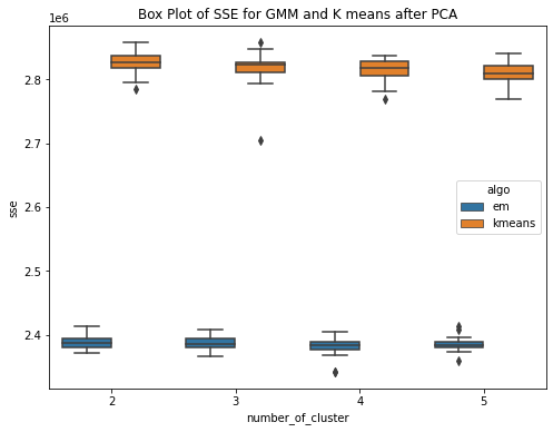
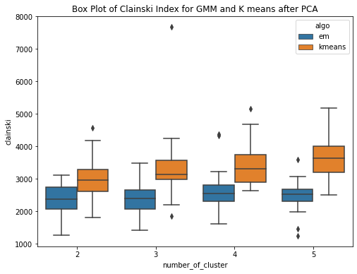
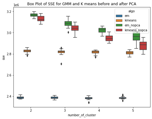
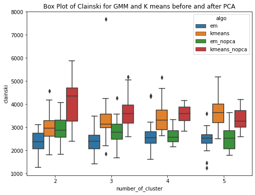
Have performed PCA over the diabetes dataset. To cover 90 percent of the variance, 24 principal components are required. So the dataset here gets reduced and now we use these principal components as data to run our GMM (EM) and kmeans algorithm. Have ran the algorithms for k = 2,3,4,5 and for each cluster the experiment is performed 20 times. PCA (Principal Component Analysis) is a method used for reducing the dimensionality of a dataset by transforming it into a lower�dimensional space while preserving most of the data variability. The transformed features resulting from PCA are linear combinations of the original features that are orthogonal to each other. PCA can help approximate a normal distribution of the data by removing redundant and correlated features and reducing the effects of outliers and noise.The aim is to improve the results. This is confirmed by the box plots. The box plot showing the within SSE between Kmeans and GMM shows the performance of GMM is much better than that of Kmeans after PCA. The median with sse is less for GMM as compared to that of the kmeans. The second plot shows the CHS score box plot for GMM and kmeans, shwoing the median value of CHS for kmeans is higher than that of the GMM. The third plot shows the comparision of within SSE for GMM and Kmeans before and after PCA. The plot shows that the sse after performing pca has much less value as compared to the previous experiments when PCA was not performed. The plot shows a huge difference in values of within sse for GMM with and without PCA and for kmeans. The fourth plot is a similar comparision but usinh CHS score as the evaluating metric. This shows that CHS score is higher before performing pca and reduces after performing PCA.
Variant of EM algorithm using different initialization technique
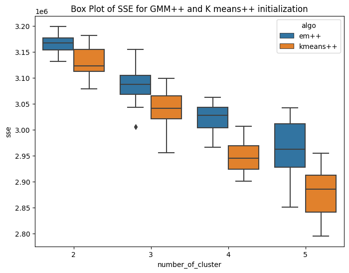
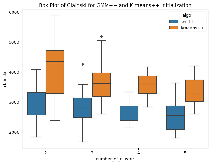
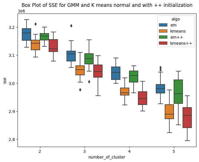
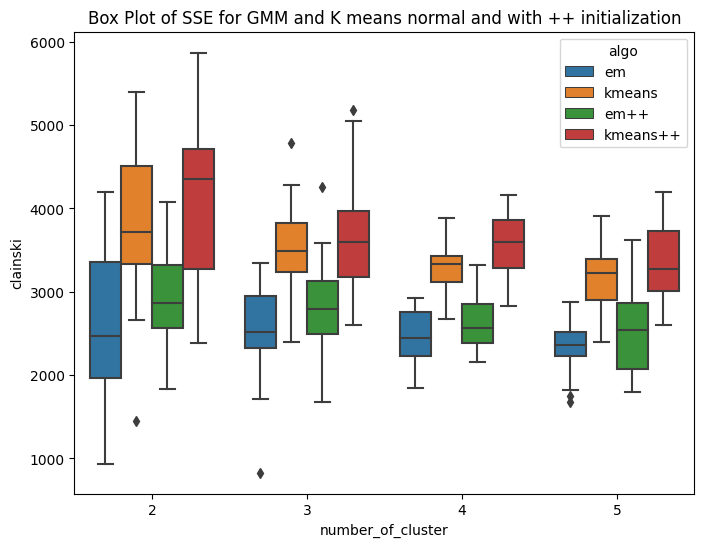
I have implemented the kmeans plus plus algorithm for number of clusters ranging from 2 to 5. The method is similar to kmeans llyod with different centroid initialization. Here the first centroid is chosen randomly from the domain of data. For rest k-1 centroids, we follow a different iterative approach. The second cluster is initialized based on the first centroid. The third centroid requires data of first two centroids. The methodolgy includes,selecting the first centroid randomly from domain of data. Then second cluster is at the farthest distance from that cluster. In this way iteratively we initialize k centroids. As the centroid initialization is not random, it is expected that the inter cluster distance will be more and intra cluster distance bewteen points and centroid will be less. The K-means++ algorithm selects the centroids in following way Step1: Choosing the first centroid at random from the data points. Step2: For each remaining data point, computing its distance to the nearest centroid that has already been chosen. Step3: Selecting the next centroid randomly from the remaining data points, with probability proportional to the squared distance to the nearest centroid. Repeating steps 2-3 until all K centroids have been chosen. The main idea behind K-means++ initialization is to select centroids that are well spread out across the data points. By selecting the next centroid from the remaining data points with a probability that is proportional to the squared distance to the nearest centroid, K-means++ initialization ensures that data points that are far away from existing centroids are more likely to be selected as new centroids. Hence the sum of square error is expected to be less. Rest the stopping conditions and other steps are similar to that of kmeans llyods. Similarly the mean matrix is initialized for GMM(EM) and same is used for K means. HAve ran this experiment for k=2,3,4,5 , running 20 times for each cluster. The first box plot shows the within Sum of square error for GMM plus plus and kmeans plus plus. It can be seen that, the median within SSE of kmeans is less than that of GMM. The second plot shows the CHS score using the new initialization technique and the value of CHS score for kmeans is higher than that of GMM. The third and fourth box plot shows the comparision of sse and CHS score for normal GMM and kmeans with the GMM plus Plus and Kmeans plus plus. The box plots shows that the median error for GMM++ is less than that of normal GMM. And similar observation is achieved for Kmeans algorithm. So by changing the initialization, the performance of the algorithms improved. This is confirmed by the CHS score as well, the median CHS score for plus plus algorithms(GMM and means) is higher than that of the median CHS score for normal initialization of GMM and kmeans